Companion Website

Prepared by: Brian A. Cohn

Feasibility Theory Reconciles and Informs Alternative Approaches to Neuromuscular Control

Journal Article, Frontiers in Computational Neuroscience (Link)

Abstract:

We present a conceptual and computational framework to unify today’s theories of neuromuscular control called feasibility theory. We begin by describing how the musculoskeletal anatomy of the limb, the need to control individual tendons, and the physics of a motor task uniquely specify the family of all valid muscle activations that accomplish it (its `feasible activation space’). For our example of static force production with a finger with seven muscles, computational geometry characterizes, in a complete way, the structure of feasible activation spaces as 3-dimensional polytopes embedded in 7-D. The feasible activation space for a given task is the landscape where all neuromuscular learning, control, and performance must occur. This approach unifies current theories of neuromuscular control because the structure of feasible activation spaces can be separately approximated as either low-dimensional basis functions (synergies), high-dimensional joint probability distributions (Bayesian priors), or fitness landscapes (to optimize cost functions).

Interactive Parallel Coordinates Visualization

A. PCA Loadings Bootstrapping Figure

Prepared by: Brian A. Cohn

Click for full size figure

Supplementary Figure: Normalized PC Loadings as task intensity increases, under different sampling sizes for PCA analysis. How do PCA loadings act when the sample number of the input dataset is impoverished? Each facet (a squared-in set of boxplots) shows how loadings change over increasing task intensity. Each facet represents a different number of samples fed to PCA. You can read each group of boxplots as a muscle’s task-dependent loading distribution. In the paper, we usd 100 replicates (PCA was run 100 times for each boxplot; each boxplot has an n=100) but for this supplemental visualization we did 1000 replicates. Each color represents a task intensity, so each cluster of boxplots (through the color palette) represents a given loading’s change over increasing distal force as the output task. The columns of faceted plots represent the number of samples fed to PCA, which were 10, 100, or 1000 (as in the paper), as well as 5000 samples.

Commands to replicate this figure on Linux or Mac.
Terminal:

$ git clone [email protected]:briancohn/space.git && cd space/pca_figure_code && R

In R:

install.packages(c('devtools','pbmcapply','dplyr','gridExtra','ggplot2'))
source('pca_bootstrapped_loadings_comparison.r')

For PC, use the Git Bash Terminal. ____

B. Muscle Task-Variance Visualization

Prepared by: Brian A. Cohn

Supplementary Figure: Visualization of activation variance for a given muscle, for a given task intensity. We find that as the intensity of the task increases, the standard deviation of all muscles decreases, where each task intensity had 10,000 points sampled. Although the muscles appear to change in variance in a similar way, different muscles have differing starting values of variance.

** Commands to replicate this figure on Linux or Mac**
In R, after the commands from above:

source('muscle_variance_over_tasks.r')

C. Figure 6 with all PCs

Prepared by: Brian A. Cohn

Supplementary Figure: Figure 6 (extended with third PC shown) PCA loadings change with task intensity. For each of 1,000 task intensities, we collected 1,000 muscle activation patterns from the feasible activation space, and performed PCA. The rows show thechanges in PC loadings, which determine the direction of PC1 and PC2 in 7-dimensional space. Note thatthe signs of the loadings depend on the numerics of the PCA algorithm, and are subject to arbitrary flips insign (Clewley et al., 2008)—thus for clarity we plot them such that FDP’s loadings in PC1 are positiveat all task intensities. These loadings (i.e. synergies) change systematically, as noted for representativetask intensities a, b, c in Fig. 5, and more so after b. This reflects changes in the geometric structure of thefeasible activation space as redundancy is lost.

Commands to replicate this figure on Linux or Mac

In RStudio, in the same working directory as above, run the file thousand_loadings.R.

D. Figure 6 with all PCs and four different input preprocessing options

Prepared by: Brian A. Cohn

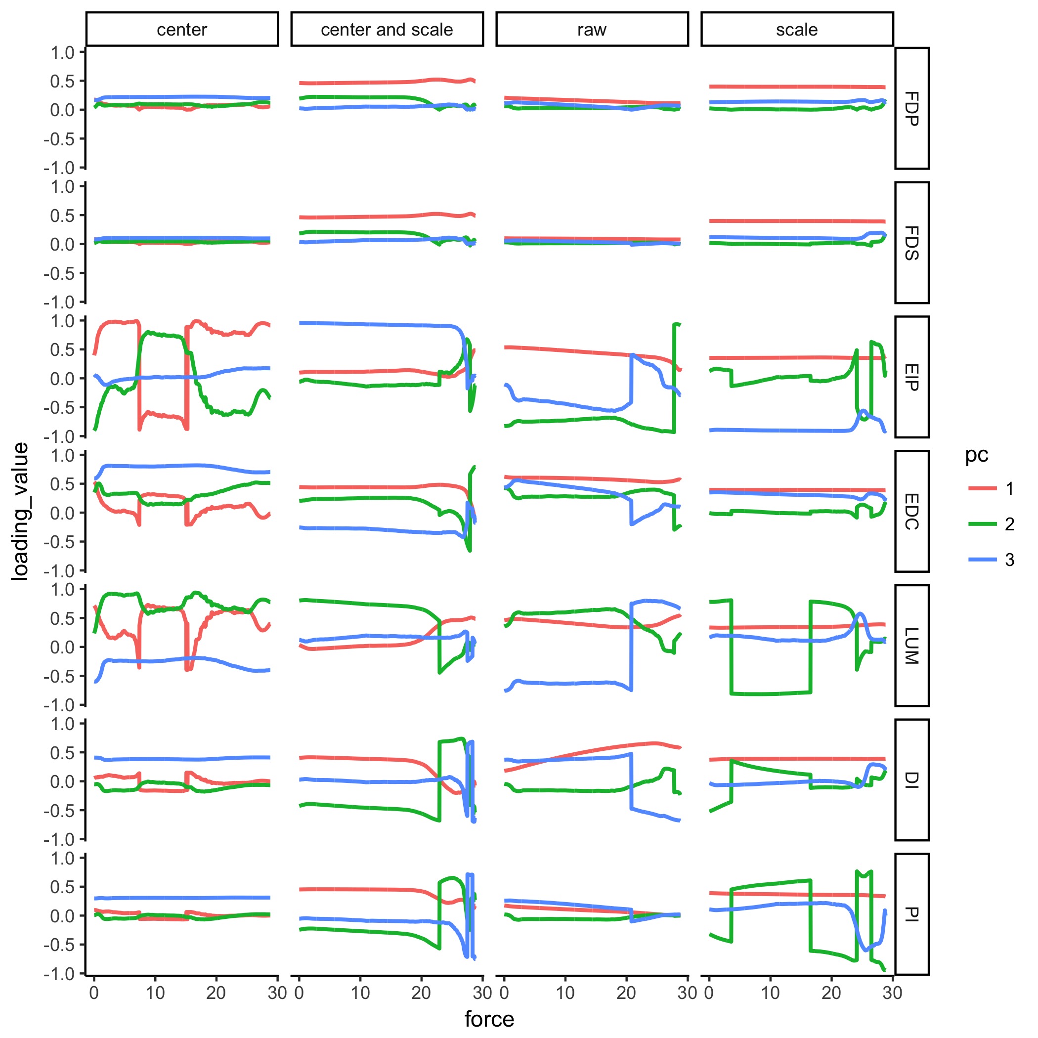
Supplementary Figure: Figure 6 with different input preprocessing The column marked “scale and center” matches that of D. and Figure 6 of the paper. We show other permutations of scaling and centering of the input data to PCA, and the results in the form of the PCA loadings for each of the three PCs. Note that all 3 PCs explain for 100% of the data. Colors do not match the pallete of the paper; see the Figure legends for each figure.

E. Same as D, but with absolute-value applied to all loadings to look at smoothing.

Prepared by: Brian A. Cohn

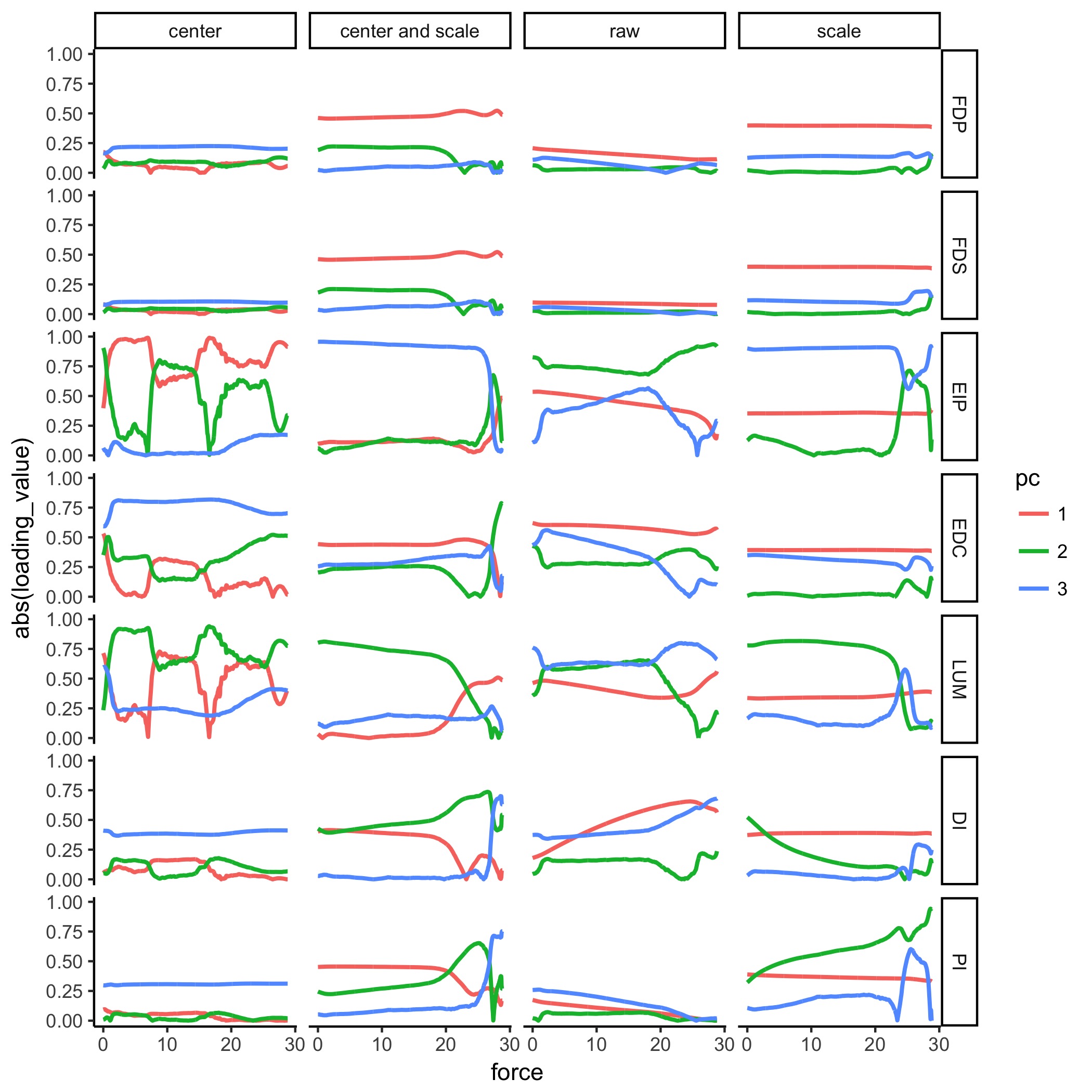
Supplementary Figure: Figure 6 We see that while it looks more smooth, some of the loadings bounce at the origin unnaturally. This is a result of calling absolute value on the loadings, where the loadings pass through the origin. Therefore, we find that showing absolute values of loadings would be misleading, as it would not highlight the actual migration of loadings.

F. Derivative of Figure 6, where pca parameters are set to scale + centering.

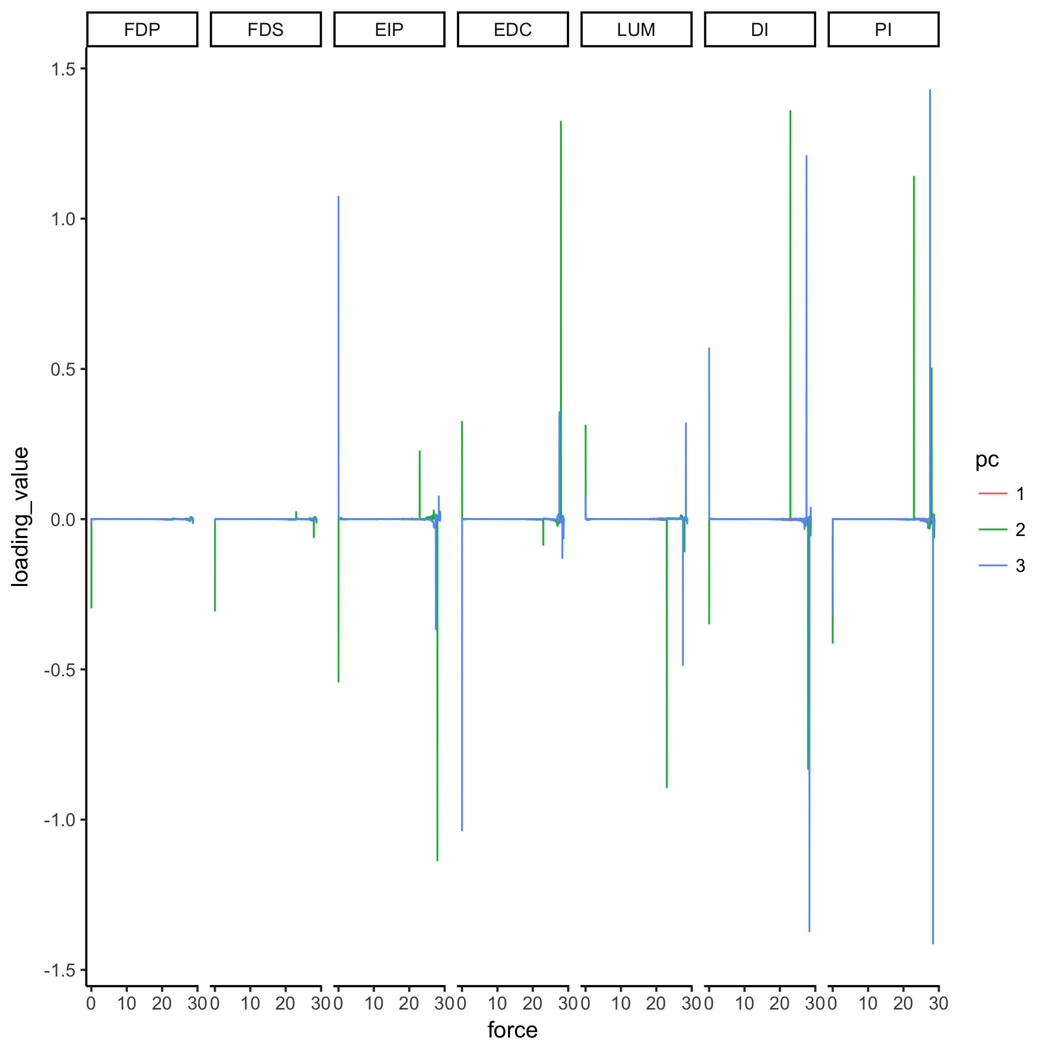
Supplementary Figure: After scaling and centering the hit and run points at each task level, we computed PCA and thereby the loadings. As in the paper, we force FDP in PC1 to keep its loading value to be positive, and propagate that flip in sign to PC2 and PC3 respectively. As a result, we do not expect to see flips in PC1—this is corroborated by our data. We can see from this derivative plot that there are instantaneously fast flips, and they typically flip up, down, and up in a cycle.

Have comments or questions about how to apply these methods to your work?

We’d be happy to help. Send us a message: [email protected]

Code to produce figures

Code to produce muscle activation patterns for a given task Parallel Coordinates in R
Histogram Heatmap in R
PCA, Loadings, and Bootstrapped Figures
Code used to calculate the size of the feasible activation space before and after post hoc constraints